Phylogeny in Brief
The term "phylogeny" refers to the study of the tree of life and the theory of common descent. When considering a group of species living today, the term also refers to the tree structure
defined by this group combined in a graphical relationship
with all of their common ancestors. In this post, I compare the basic classification methods of early biologists with the
methods developed over recent decades inspired by the dramatic
increase in availability of genetic sequence data.
A phylogeny is a tree structure
that defines a history for the species of the past that are ancestral to a
group of species living today. For
example, consider the great apes, consisting of humans (Homo), chimpanzees
(Pan), gorillas (Gorilla), and orangutans (Pongo):
Ape Phylogeny

(Graphic borrowed from www.mailund.dk)
We see that the common ancestor of
humans and chimpanzees is placed in a position more recent than that of humans,
chimpanzees, and gorillas. In this
phylogeny, the orangutan is the outgroup, the species whose nearest ancestor to the rest of the species predates the rest
of the common ancestors, i.e., the species first to diverge from the rest of the group.
Before the study of phylogeny (and
more generally, the study of evolution), it was widely believed that the
species we see today always existed in their current form. Fish were always fish, trees were always
trees, bears were always bears, and humans were always humans. Indeed, this interpretation seems simple and intuitive. But Darwin's Theory of Evolution suggested that species could evolve with new traits arising in populations as they increased the fitness of living beings. Also, new species could arise when a living species separated into two or more branches that started to evolve independently. One conclusion drawn from the
study of phylogeny is that humans and apes have a common ancestor, a belief
that becomes easily caricatured as “People came from monkeys!”
Strictly speaking, humans did not
descend from “monkeys.” Rather, the
theory of evolution states that humans, apes, and other primates all had a
common ancestral species several million years ago. In the current work, I try to briefly explain
how this counter-intuitive theory has become dominant in the field of
evolutionary biology.
History
Theory of Common Descent
With the publication of The Origin of Species, Charles Darwin
presented a radically new idea describing the history of all life on this
planet. According to this theory,
species would evolve: small changes
in a species that were favored by the environment would come to dominate the
species. For example, a species of finch
that lived on an island on the ground might find it more useful to have a
short, fat beak. With a shorter beak,
the finch would find it easier to feed on seeds it could collect, and its
survival rate would improve. A species of finch on a different island might find
a habitat with more trees. In such a
habitat, a long, narrow beak might be better at reaching insects in
hard-to-reach crevices. On a third island,
a third type of beak might be favored.
It is important to note that the
species doesn’t choose what type of beak it has, nor does it intentionally pass
on genes containing the adaptation. Rather,
the entire process is passive. The
dominance of a new characteristic is implied by the survival rate alone. Or to be more precise, the dominance of a gene in the population grows as a
function of the gene’s propagation rate.
Once a gene establishes a higher survival rate in the population, its
ascension to a position of dominance is a mathematical inevitability.
Genetic mutability is the
observable fact that the genetic composition of a species can change over
time. (This fact is most readily
observable with quickly evolving species such as bacteria and viruses.) But mutability is only part of the theory of
evolution. Genetic mutability does not,
by itself, imply common descent.
Consider, as an example, the appearance of uniforms in the sport of
professional baseball. Each franchise
tends to make small variations in the appearance from year to year. And one could trace these changes if one had
access to older uniforms or photos or drawings thereof. But the fact that each franchise’s uniforms
can change does not, by itself, imply that there was a single franchise at the
beginning of the baseball league.
This brings us to the concept of common descent. When Darwin famously toured the Galapagos
Islands on the HMS Beagle, he observed similar species of finches on various
islands. Struck by the similarities of
many of their features, Darwin postulated that they had all descended from a
common ancestral finch. But when the ancestral species settled on the several
islands, the descendants diverged in
the sense that different characteristics became dominant in different
locations.
As species diverge, interbreeding
between the various populations can become more and more difficult, for a
variety of biological and geographical reasons.
After enough time passes, the original populations are no longer
biologically compatible in a mating sense.
This process of divergence is called speciation,
and the diverse descendant populations are called species.
The Tree of Life
The concept of speciation led to a
revolution in how scientists viewed our natural history. No longer did scientists view species as
eternally fixed in form and function, but rather, variability was allowed into
the theory. Furthermore, the concept of
species extinction was first raised
by the systematic investigation of fossils, the discovery of which was
proceeding apace in the 19th Century.
The diversity of life had been
recognized since antiquity and, indeed, the possibility of meaningful
classification was always apparent.
Humans have long recognized the differences between birds, mammals, and
fish, for example, and have understood that certain groups of animals are more
similar to each other than any is to species outside the group. Thus we have
carnivores and ungulates, insects and crabs, lizards and snakes, etc. It became apparent that a natural taxonomy
could be constructed on all living species, where dividing points in the
taxonomy represented major differences between groups of species.
With the introduction of the theory
of common descent, such a classification drew a natural meaning in terms of the
shared evolutionary history. Let us
consider all the descendants of some species that existed hundreds of millions
of years ago. If we traced the species through time, we could model any
speciation event as a node, with a path leading away from that event
representing a new species.

As the descendant species
themselves radiate geographically and undergo their own speciation events, the
new paths will lead to new nodes and new divergences.

If we trace this
process throughout the millennia, the tree structure can become quite elaborate. In 1866, Ernst Haeckel suggested the tree
structure below, dividing living species into three kingdoms: Plants, Protists,
and Animals.
Haeckel’s Tree of Life

Reconstruction Methods
So far, we’ve considered how
evolution may have proceeded. But we have
no witnesses to the millennia of evolutionary history. Well, sure we have some fossil records that
may represent ancestral species to what we see today, but at best the fossil
record is incomplete. Today’s biologist
will need to rely on the powers of inference to determine what the most likely
explanation would be.
Note that I am using the language
of likelihood here. Science does not
reveal absolute truths, but provides theories, along with a measure of
confidence in the theory. Any phylogeny
is a theory of what kind evolutionary history is shared by a set of species
that live today. So if we are going to
tackle the task of building a tree like the one above, we need to have a
well-defined protocol for doing so, with a sound basis in scientific logic.
I will briefly present two general
methods for building phylogenies. First,
we’ll consider the character-based method, which was used by Darwin and Haeckel
and early taxonomists. In this method,
characteristics of types of living species (plant vs. animal, cold blooded vs.
warm blooded, exoskeleton vs vertebrate, etc.) are used to divide the
species. Taxa are grouped in the tree
based on the theory that major changes in structure happen rarely. Thus the tree structure should reflect this
principle of parsimony.
In the second method, molecular
sequence data is used to generate a tree.
This approach is more mathematical than the character method. At its core is a mathematical model of how
DNA and protein sequences evolve through time, accumulating tiny changes in the
code that do not affect protein function.
We then apply statistical theory and use the power of modern computing
to find a tree structure that best fits the data we are considering.
Tree Topologies
To select a phylogeny, we need to
select a) a tree topology, and b) branch lengths for the tree. Essentially, the topology of the tree is its
shape. For our purposes, each branch
will also have a length associated with it, representing the time between
speciation events. Generally speaking,
the process of fitting a phylogeny to sequence data (or, indeed, to any kind of
data), has two parts: 1) selecting a toplogy, and 2) selecting branch
lengths. For a given tree topology and a
model of evolution, finding the optimal branch lengths is a straightforward
(albeit computationally expensive) optimization problem. (Felsenstein.)
The computational issues in
phylogeny fitting arise from the number of tree topologies, which increases
exponentially with the number of taxa (taxa
are the species living today forming the base of the tree). Let us consider why this happens:
Let’s let n be the number of taxa under consideration. Then a phylogeny with n taxa will have (n-2) internal nodes and thus (2n-3)
branches. If we add another taxon to the
tree, there are (2n-3) branches that
could be split by the new branch leading to the new leaf, and each of these
insertion points would lead to a different topology. If we let T(n) be the number of topologies, we see
that be the number of topologies, we see
that T(n+1) = (2n-3) T(n). Since T(3)
= 1, the formula for T(n) is T(n)=(2n-5)!! (Here the
double factorial notation x!! is
defined for any odd value of x to
mean x!! = (x*(x-2)*(x-4)*…*3*1). In other words, the number of possible
topologies increases very quickly as the number of taxa increases.
The obvious approach to finding an
optimal phylogeny would be to find the optimal branch lengths for each
topology. But it quickly becomes
computationally infeasible given the rapid growth of T(n). An exhaustive search
over all topologies is quickly infeasible as n increases. For example,
10!! = 3840, which is a manageable number of trees for a program to evaluate,
but 20!! = 3.72 * 109, and 30!! = 4.28 * 1016. Thus, exhaustive searches are impracticable
for all but the smallest phylogenies.
Character-based methods
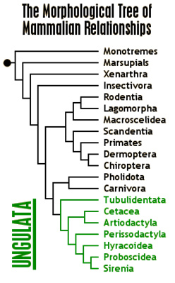
The tree below (graphic from http://www.ultimateungulate.com/whatisanungulate.html)
shows a mammalian phylogeny based on a traditional, character-based
method. In such an approach, high-level
phenotypes are presumed to be preserved.
Thus all species sharing a trait are believed to make a clade, i.e. a subtree with a common
ancestor that excludes species that don’t have said trait. For example, placental mammals are generally
believed to comprise a clade in the phylogeny of mammals. In the tree above, the egg-laying mammals
(monotremes) and the pouch-using marsupials are outgroups to the rest of the
tree, all of which are placental mammals.
Also highlighted in this tree are the ungulates: a collection of orders
included all mammals with hooves, and some orders (such as cetaceans) believed
to be derived from ungulates.

Unfortunately for taxonomists, most
useful characters are not so easily defined in a way that makes them
cladistics. As with the cetaceans above,
a sub-clade within a clade may lose the evidence of the ancestral
character. Also, there is the problem of
parallel evolution. Useful biological
features may have arisen along separate lines.
(A simple example of this would be the trait of winged flight, which
exists within birds, mammals, and insects.)
Genetic revolution
The discovery of the structure of
DNA in the mid-20th century led to a new way to compare
species. By comparing the sequences of
homologous proteins from different species, one could see that each species had
witnessed functionally neutral mutations through history. A typical gene has thousands of base pairs in
its coding region, so the mutation of a small number of base pairs in the gene
can often be neutral with regard to the gene’s expression.
There are a number of different types of DNA mutations. A single base pair may vary. Also, an entire stretch of the genome may be
duplicated and repeated, or it may drop from the genome altogether. But, presuming not too many mutations have
happened, it is possible to align
sequences from regions that have been relatively conserved over time.
Sample Multiple Sequence Alignment
(Grahpic borrowed from http://users.ugent.be/~avierstr/principles/aligning.html)
In this graphic, the four letters A, C, G, and T represent the four DNA bases
adenine, cytosine, guanine, and thymine.
The ‘-‘ characters or ‘gaps’ are inserted into the sequences in the
alignment to indicate points where a sequence has lost that particular base
pair from its sequence. (Alternatively,
in a column where most of the species have a gap, the interpretation is that
some of the sequences have had an extra base pair inserted.)
If we focus on columns that have no
gaps, we can model the changes in the sequence according to a fairly simple
random model.
Random Walks
Let us suppose we have a tourist
walking through a museum with exhibits in several different rooms. We could track the progress of the tourist
and make a note every fifteen minutes of his location in the museum. This kind of process is known as a random walk, a special kind of random
process. If the museum had a proscribed
order for viewing exhibits, this pattern might be predictable. But let us suppose that the museum consists
of unrelated exhibits, and that our visitor is choosing his next exhibit at
whim. Let’s also assume that the amount
of time he might spend in a given exhibit is itself random. Our list of rooms, observed over time,
represents the output of a random process. This kind of process, where our
observations are of chosen from a finite number of states, but the odds of
change vary as time varies, is called a stochastic
process.
The example of the museum visitor
has a feature which we may not want for modeling evolution. Namely, the museum visitor is likely to spend
a predictable amount of time at each exhibit.
In other words, the longer a visitor has already spent at a certain
exhibit, the more likely he is to move on.
DNA mutation is, however, memoryless
in the sense that the probability of a mutation at a given time is independent
of how long it has been since the previous mutation. An example of a memoryless random system in
real life is a roulette wheel. Whether one has seen the number ‘25’ show up
five times in a row or whether the wheel has been spun 2,000 times without
seeing a ‘25’, the probability of a ‘25’ on the next spin will be the same
(1/38 on a well-balanced American wheel).
A stochastic process that is
memoryless can be called (if a few other conditions also hold) a Markov process. With a Markov process,
the probability of any state change can be expressed as a function of the
amount of time elapsed between observations.
To relate to our museum visitor, if i
and j represent two rooms of the museum, and if t is an amount of time, then we can define pij(t) to be the probability that if the
visitor starts in room i, the probability
that he is in room j after t units of time.
Using the alignment as the next
point of departure, it’s possible to develop a dissimilarity measure on the
species based on which sites are witnessing mutations. The general idea is that one can estimate how
much evolutionary time has passed between a pair of species as a function of
how similar (or rather, how dissimilar)
their sequences are. The more time that
passes, the more divergence you’ll see between the pair. When all of the sites are considered at once
(i.e., when all of the columns of the alignment are considered), we obtain an
estimate for pij(t).
As t approaches infinity, the
values of pij(t) will converge to a limiting value, pj
(which in fact does not depend on i.) This fact allows us to make an estimate of
the value of t that best fits the
data.
Heuristics
Given the enormous number of tree topologies possible, there
is a need for a way to select one of the topologies without testing all of
them. Many computer algorithms have been designed for this task. The most popular methods for doing this with
very large data sets are distance methods.
They work by using dissimilarity information on the set of taxa to
generate a metric (distance function) on the taxa. Then, a tree is constructed such that the
evolutionary distances implied by the tree serve as a good approximation to the
observed distances. Computer algorithms
have been designed that can do this in computational time polynomial in n.
The most popular distance method is an algorithm known as
Neighbor-Joining. It works recursively:
- By scanning the input matrix M, find a pair of taxa, x, y that are to be neighbors in the tree.
- Reduce the set of taxa by defining a new taxon x-y, to replace x and y.
- Calculate a new reduced matrix M’on the reduced set of taxa.
- Recursively solve the problem for M’ to build a tree T’.
- Build the tree T by replacing attatching the node x-y in T’ to the nodes x and y.
This entire process can be done in computational time
proportional to n3. Once an initial tree topology has been
selected, this can serve as starting point for whatever statistically-based
search process that may be desired.

Tree Rearrangements
With an initial topology T in hand, the tree builder now needs
methods for making slight tweaks to the topology, to generate other topologies
“close” to T for evaluation. There are several methods for doing this:
- Nearest neighbor interchange: in a binary tree (i.e., a tree where each internal node is met by exactly three branches), each internal branch defines four subtrees, two on each side of the branch. A nearest neighbor interchange swaps one of the subtrees on one side of the branch for one of the subtrees on the other side of the branch.
NNI rearrangement

- Sub-tree pruning and regrafting: similar to the reinsertion method above, except that instead of re-inserting just one taxon, an entire subtree is removed and re-inserted. In the figure below, the subtree S is moved past the other subtrees T1, T2, … Tk.

- Tree bisection and resection: an internal branch is deleted from the tree, creating two smaller trees. Then the trees are re-connected by grafting part of a branch from one tree to part of a branch from the other tree. (All pairs of insertion points are tested.)
TBR rearrangement

Graphic from http://en.wikipedia.org/wiki/Tree_rearrangement
It is common to pick one of the methods
above to generate a new list of topologies, which are then each evaluated. If a new topology is deemed superior, it is
then selected as the initial point for a new search. The process is repeated until an optimal
point is reached.
Likelihood Methods
This raises the question of how we
score topologies. The most common method
is to use a likelihood approach. In this
approach, we consider the likelihood score of each topology: given a model M, data D, tree T and probability
function P, the likelihood score is
L(M,D)=P(D|M,T)
i.e., it’s the probability of seeing the
given data, given the model of evolution used. For a given topology, finding
the branch lengths which optimize this function is itself a problem that can
require a good deal of computation. But
at long as the number of topologies is limited in size, these computations can
be done in a reasonable amount of time.
So, to summarize, the
molecular approach is to
1.
Given an alignment of homologous DNA or protein
sequences, build a distance matrix D
generated by the pairwise dissimilarities.
2.
From D,
build a tree T0 such that
the metric implied by T0
serves as a good approximation to D.
3.
Use T0
as the initial point and use toplogical rearrangements (NNIs, SPRs, or
TBRs) to search through candidate tree topologies. For each tree topology, find branch lengths
that optimize the likelihood function, and choose the topology whose likelihood
is optimal among the candidate trees.
Repeat search until no improvement in likelihood function is found.
It is true that the tree selected
by Step 3 will not necessarily be optimal over all possible trees. But the advantage of using likelihood as the
method here is that relative strengths of alternative trees is implicitly
expressed by the likelihood scores. The
likelihood score not only points to a topology, but provides a way to measure
just how much confidence we should have in that topology.
Impact of molecular information
With the general framework outlined
above, statisticians and computer scientists have devised a number of methods
to evaluate many possible phylogenies for species living today. In many cases, the data generated by
sequencing proteins and DNA from living species has forced scientists to
rethink their earlier phylogenies. All
sorts of phylogenetic questions have been revisisted, such as
- The early history of apes: which species diverged first from the other two, humans, chimpanzees, or gorillas?
- How many kingdoms are there in the tree of life? That is to say, since the plant, animal, and fungal kingdoms are well-defined, how do the various protists and bacteria fit into the mix?
- How do extinct classes of species (such as dinosaurs) relate to those living today? In particular, are reptiles the nearest living relatives of dinosaurs, or do the birds serve as a more likely candidate?
With the advances in sequencing
technology in the past twenty years, and the progress of projects to sequence
the entire genomes of humans and several other species, we now have enough data
to evaluate questions like these with far more sophisticated statistical
methods than were available in the past.
Thus, the profusion of data has led to much stronger statistical support
for various hypotheses than were possible in even the recent past.
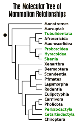
As a final point, consider what
taxonomists now think to be the shape of the mammalian tree, and how the
ungulates have been affected by the accumulation of genetic data. The molecular data simply do not support the
theory that ungulates form a clade.
Rather, the similar hoof shape is something that has separately evolved
several times in the long history of mammals.

References
A basic primer on phylogenies
The foundational work on likelihood by Joe Felsenstein
More about Neighbor-Joining